Linear Regression in R
Given a set of noisy data points, such as the following, how can we find the best fitting linear model?
x <- c(1, 2, 3, 4, 5, 6)
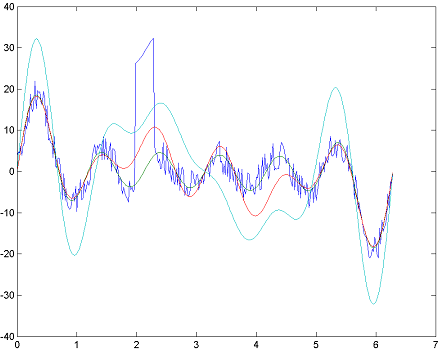
t <- seq(from = 0, by = 0.02, to = 2*pi)
A <- cbind(sin(t), sin(2*t), sin(3*t), sin(4*t), sin(5*t), sin(6*t))
e <- -4+8*runif(length(t),min=-1,max=1)
e[100:115] <- 30
y = A%*%x + e
plot(t, y, 'l')
Various packages in R support linear regression models, such as stats (for least-squares) and quantreg (for quantile regression):
library(stats)
res1 <- lm(y ~ A)
lines(t, res1$fitted.values, col='green')
qr.solve(A, res1$fitted.values)

library(MASS)
res2 <- rlm(y ~ A)
lines(t, res2$fitted.values, col='red')
qr.solve(A, res2$fitted.values)

library(quantreg)
res3 <- rq(y ~ A)
lines(t, res3$fitted.values, col='darkred')
qr.solve(A, res3$fitted.values)
How can we implement these techniques in R to better understand how they work?
Here are two implementations that use convex optimization:
# Ordinary Least Squares regression
ols <- function(x, y) {
obj <- rep(1, length(x) +2 )
obj[c(1,2)] <- 0
eye <- diag(length(x))
bvec <- y
Amat <- cbind(x, rep(1, length(x)), eye)
Dmat <- matrix(0, length(x)+2, length(x)+2)
diag(Dmat) <- 1;
Dmat[1,1] <- 1e-7
Dmat[2,2] <- 1e-7
dvec <- rep(0, length(x)+2)
res <- solve.QP(Dmat,dvec,t(Amat),meq=length(x), bvec=bvec)
yhat <- res$solution[1]*x +res$solution[2]
lines(x, yhat, col='blue')
}

# Ordinary Least Absolute Deviation regression
olad <- function(x, y) {
obj <- rep(1, length(x)+2)
obj[c(1,2)] <- 0
eye <- diag(length(x));
mat1 <- cbind(x, rep(1, length(x)), -1*eye)
mat2 <- cbind(x, rep(1, length(x)), eye)
mat <- rbind(mat1, mat2)
dir <- c(rep("<=", length(x)), rep(">=", length(x)))
rhs <- c(y, y)
types <- c(rep("C", length(x)+2))
max <- F
res <- Rglpk_solve_LP(obj, mat, dir, rhs, types = types, max = max)
yhat <- res$solution[1]*x +res$solution[2]
lines(x, yhat, col='green')
}
Regression using L1, L2 and L∞ norms source.
How do these implementation work? What are their limitations?