Three forecasting techniques

15 Feb 2012

How well are we doing when forecasting for online ads at Adap.tv? Can we do better? To start answering such questions, I used R to experiment with three well-known forecasting techniques and used an hourly metric (transformed for data privacy) across all ads for seven days (Feb 1-Feb 7) as my training data set. Then I use each of the techniques to predict for the eight day (Feb 8), and compare the predicted values with actual data. Here’s a synopsis of the three:

Exponential Weighted Moving Average (EWMA)_

Strictly speaking, the smoothing filter that we currently use at Adap.tv for forecasting is not EWMA, but more like Weighted Moving Average. EWMA is defined by:

$S_{t} = \alpha \times (Y_{t-1} + (1-\alpha) \times Y_{t-2} + (1-\alpha)^2 \times Y_{t-3} + ... + (1-\alpha)^k \times Y_{t-(k+1)}) + (1-\alpha)^{k+1} \times S_{t-(k+1)}$ (ref)

So, if a = 0.9, S[t] = 0.9 ( y[t-1] + 0.1*y[t-2] + 0.01*y[3] … 1e-6*y[t-7]) would be an implementation of EWMA. Instead, our implementation is be: S[t] = 0.9 ( y[t-1] + 0.9*y[t-2] + 0.81*y[3] … 0.531441*y[t-7]) / (0.9+…). The critical difference is in the way past data is weighted - with EWMA data in remote past is heavily penalized, whereas, comparatively, in our implementation it is not.

Fig. 1 below shows a plot that forecasts our metric for Feb 8 using Weighted Moving Average akin to our implementation. The metric forecasted for Feb 8 was 68392533 whereas observed value was 63868927, giving an absolute difference of ~7.1%. The absolute hourly differences lie between 0.6-29%.

Fig. 1, “Weighted moving average”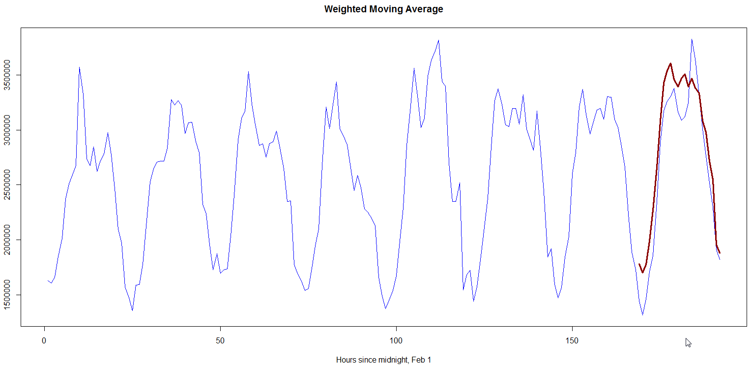

Harmonic regression_ Harmonic regression attempts to find the best-fitting periodic signals that can

characterize a time series. For example, we a time series may be represented by a linear sum of sinusoids:

$\frac{a_0}{2} + \sum_{n=1}^\infty \, [a_n \cos(nx) + b_n \sin(nx)]$ (ref)

Generally, a combination of Fourier transform and least-squares regression in used to find the harmonics who linear sum best fit training data. In my experiment, I used the top seven harmonics with highest power density (i.e. contribution to the model), and then used linear regression to find their amplitudes. Fig. 2 shows the model (in red) and actual data (in blue). The forecast for Feb 8 was 60476559 whereas the observed value was 63868927, giving an absolute difference of ~5.3%. The absolute hourly differences lie between 0.05-25%.

Fig. 2, “Harmonic regression” 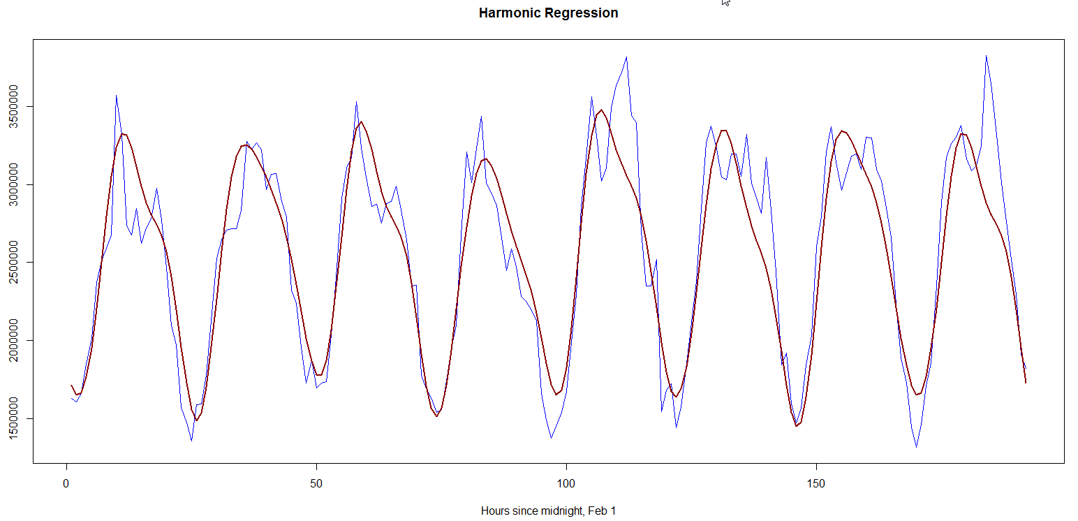](/assets/images/harmreg2.png)

Holt-Winters method_

Holt-Winters method augments EWMA to account for data trends and seasonality.

$\begin{align} s_0& = x_0\ s_{t}& = \alpha \frac{x_{t}}{c_{t-L}} + (1-\alpha)F_t\ b_{t}& = \beta (s_t - s_{t-1}) + (1-\beta)b_{t-1}\ c_{t}& = \gamma \frac{x_{t}}{s_{t}}+(1-\gamma)c_{t-L}\ F_{t+m}& = (s_t + mb_t)c_{(t+m) \pmod L}, \end{align}$ (ref)

The model I used assumes that the seasonal component is additive (instead of being multiplicative). Fig. 3 illustrates the breakdown of seasonality, trend and randomness in the data, Fig. 4 contrasts observed data with predicted data (note that the prediction start after one period, and the phase lag in predicted data), while Fig. 5 shows Holt-Winters prediction for Feb 8 versus observed data. The forecasted metric for Feb 8 was 63801332 whereas observed value was 63868927, giving an absolute difference of ~0.11%. The absolute hourly differences lie between 1.3-20%.

Fig. 3 ](/assets/images/holtwintersdecomposition2.png)

Fig. 4 ](/assets/images/holtwintersfit2.png)

Fig. 5 ](/assets/images/holtwintersprediction2.png)

TO-DO

Compare these models for other data set time ranges (weeks, months, quarters)
Compare these models for other metrics by sub-populations (e.g. by view domains)
Test for stationarity, or otherwise heteroscedasticity, across models and data sets. This may be critical since non-stationary time series should not be modeled with moving average methods
Compare models when data is uniformly sampled

Posted by Umayr Hassan